Ordinal Regression Tutorial
UCLA Dataset
Let us first explain the API of myfm.MyFMOrderedProbit
using UCLA dataset.
The data description says
This hypothetical data set has a three level variable called apply, with levels “unlikely”, “somewhat likely”, and “very likely”, coded 1, 2, and 3, respectively, that we will use as our outcome variable. We also have three variables that we will use as predictors: pared, which is a 0/1 variable indicating whether at least one parent has a graduate degree; public, which is a 0/1 variable where 1 indicates that the undergraduate institution is public and 0 private, and gpa, which is the student’s grade point average.
We can read the data (in Stata format) using pandas:
import pandas as pd
df = pd.read_stata("https://stats.idre.ucla.edu/stat/data/ologit.dta")
df.head()
It should print
apply |
pared |
public |
gpa |
|
|---|---|---|---|---|
0 |
very likely |
0 |
0 |
3.26 |
1 |
somewhat likely |
1 |
0 |
3.21 |
2 |
unlikely |
1 |
1 |
3.94 |
3 |
somewhat likely |
0 |
0 |
2.81 |
4 |
somewhat likely |
0 |
0 |
2.53 |
We regard the target label apply as a ordinal categorical variable,
so we map apply as
y = df['apply'].map({'unlikely': 0, 'somewhat likely': 1, 'very likely': 2}).values
Prepare other features as usual.
from sklearn.model_selection import train_test_split
from sklearn import metrics

X = df[['pared', 'public', 'gpa']].values
X_train, X_test, y_train, y_test = train_test_split(X, y, test_size=0.2, random_state=42)
Now we can feed the data into myfm.MyFMOrderedProbit.
from myfm import MyFMOrderedProbit
clf = MyFMOrderedProbit(rank=0).fit(X_train, y_train, n_iter=200)

p = clf.predict_proba(X_test)

print(f'rmse={metrics.log_loss(y_test, p)}')
# ~ 0.84, slightly better than constant model baseline.
Note that unlike binary probit regression, MyFMOrderedProbit.predict_proba()
returns 2D (N_item x N_class) array of class probability.
Movielens ratings as ordinal outcome
Let us now turn back to Movielens 100K tutorial.
Although we have treated movie ratings as a real target variable
and used MyFMRegressor, it is more natural to regard them
as ordinal outcomes, as there are no guarantee that the difference between rating 4 vs 5
is equivalent to the one with rating 2 vs 3.
So let us see what happens if we instead use MyFMOrderedProbit to predict the rating.
If you have followed the steps through the previous ‘’grouping’’ section,
you can train our ordered probit regressor by
import numpy as np
from sklearn.preprocessing import MultiLabelBinarizer, OneHotEncoder
from sklearn import metrics

import myfm
from myfm.utils.benchmark_data import MovieLens100kDataManager

FM_RANK = 10

data_manager = MovieLens100kDataManager()
df_train, df_test = data_manager.load_rating_predefined_split(fold=3)

FEATURE_COLUMNS = ['user_id', 'movie_id']
ohe = OneHotEncoder(handle_unknown='ignore')

X_train = ohe.fit_transform(df_train[FEATURE_COLUMNS])
X_test = ohe.transform(df_test[FEATURE_COLUMNS])
y_train = df_train.rating.values
y_test = df_test.rating.values

fm = myfm.MyFMOrderedProbit(
    rank=FM_RANK, random_seed=42,
)
fm.fit(
    X_train, y_train - 1, n_iter=300, n_kept_samples=300,
    group_shapes=[len(group) for group in ohe.categories_]
)
Note that we have used y_train - 1 instead of y_train,
because rating r should be regarded as class r-1.
We can predict the class probability given X_test as
p_ordinal = fm.predict_proba(X_test)
and the expected rating as
expected_rating = p_ordinal.dot(np.arange(1, 6))
rmse = ((y_test - expected_rating) ** 2).mean() ** .5
mae = np.abs(y_test - expected_rating).mean()
print(f'rmse={rmse}, mae={mae}')
which gives us RMSE=0.8906 and MAE=0.6985, a slight improvement over the regression case.
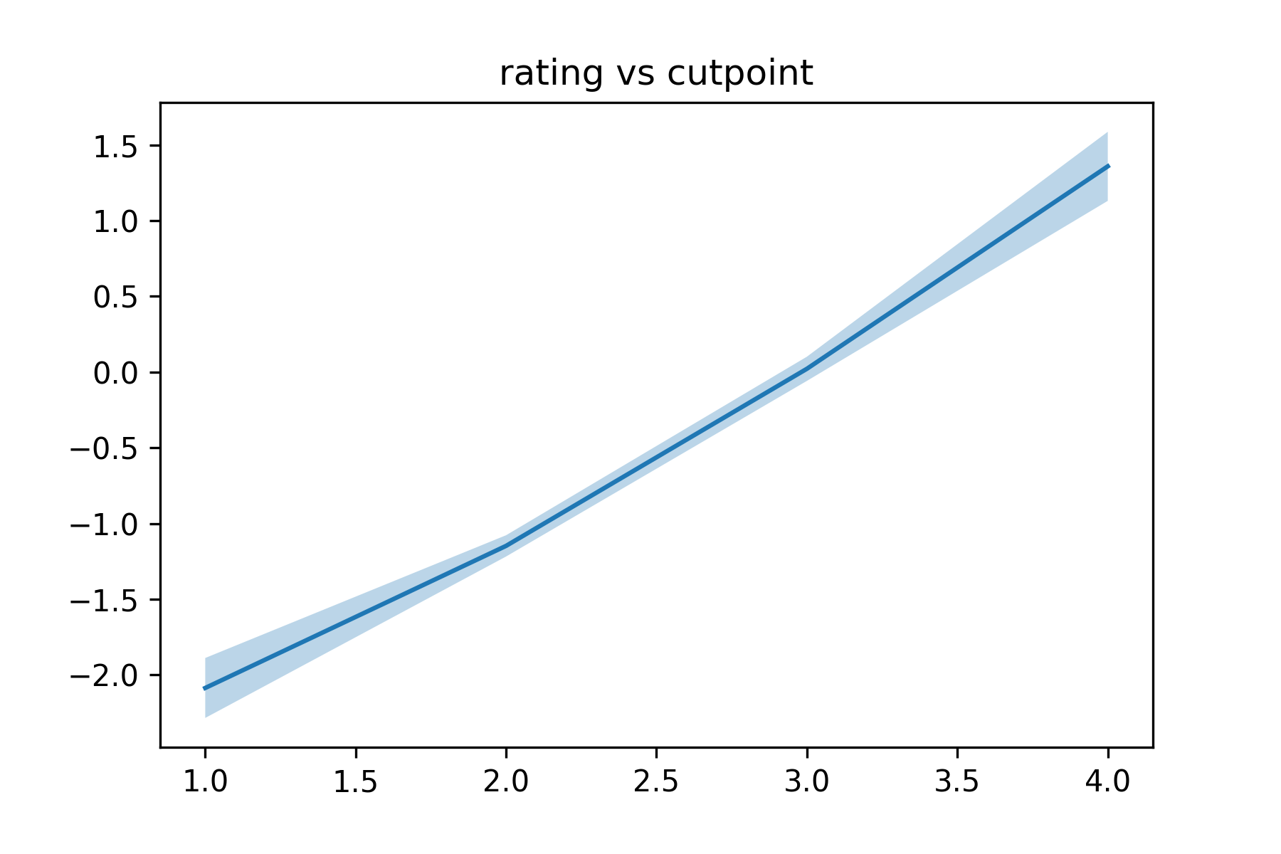
To see why it had an advantage over regression, let us check the posterior samples for the cutpoint parameters.
cutpoints = fm.cutpoint_samples - fm.w0_samples[:, None]
You can see how rating boundaries vs cutpoints looks like.
from matplotlib import pyplot as plt
cp_mean = cutpoints.mean(axis=0)
cp_std = cutpoints.std(axis=0)

plt.plot(np.arange(1, 5), cp_mean);
plt.fill_between(
    np.arange(1, 5), cp_mean + 2*cp_std, cp_mean - 2 * cp_std,
    alpha=0.3
)
plt.title('rating boundary vs cutpoint')
This will give you the following figure. The line is slightly non-linear, which may explain the advantage of the formulation in ordinal regression.
You can also improve the performance for Movielens 1M & 10M dataset. See our examples directory.